System Identification for Smart Maintenance: A Practical Example


Paula Pico
Juan Pablo Valdes
Overview
This blog provides starter python code examples for doing system identification in the context of anomaly detection. The blog is aimed at practitioners interested in exploring system identification libraries and learning about the added value of using the Quaisr platform for cases like anomaly detection.
An entry point: SystID and fault detection with SIPPY and Quaisr
SIPPY is an open-source Python package aimed at performing SystID of dynamic systems. Its simplicity of use and navigation is based on the short and easy, yet flexible lines of code needed to define and set up a case study at the beginner or expert level. Suppose we have a physical asset and would like to be alerted if its normal operational mode has been disrupted by structural integrity damage. For this illustrative example, let’s imagine we simulate input–output signals spanning 450s of operation through a high-order model, which usually characterises complex systems, such as processes with dead times, inverse responses, and subprocesses in series. This process model template can represent actual operation of engineering components such as direct current motors and process plants. Within the time period defined, the system underwent a behavioural change (i.e. the coefficients of the process model changed) during the interval 150 - 300s and then reverted back to its initial operational mode; are we able to detect this change? The answer, of course, is yes. The key to achieve this involves three steps:
- Importing all relevant packages and creating our output signals given a particular input vector,
u(t). In this example, the user creates the synthetic output signal,y(t), from a simple time-series model, with a sampling time of 1s, and modify the gain,Kp, and time constant,taup, from 3.0 and 5.0 to 5.0 and 7.0, respectively, to simulate the anomaly in operation:
import sippy
import control.matlab as cnt
import numpy as np

import time

import numpy as np
import pandas as pd
import matplotlib.pyplot as plt

from scipy.integrate import odeint
from scipy.optimize import minimize
from scipy.interpolate import interp1d

sampling_time = 1.0

# define process model (to generate process data) Check out http://apmonitor.com/pdc/index.php/Main/FirstOrderOptimization for further details
def process(y, t, n, u, Kp, taup):
  # arguments
  #  y[n] = outputs
  #  t    = time
  #  n    = order of the system
  #  u    = input value
  #  Kp   = process gain
  #  taup = process time constant

  # equations for higher order system
  dydt = np.zeros(n)
  # calculate derivative
  dydt[0] = (-y[0] + Kp * u) / (taup / n)
  for i in range(1, n):
      dydt[i] = (-y[i] + y[i - 1]) / (taup / n)
  return dydt

# specify number of steps
ns = 450
# define time points
t = np.linspace(0, ns, ns + 1)
delta_t = t[1] - t[0]

# define input vector
u = np.zeros(ns + 1)
u[5:20] = 1.0
u[20:30] = 0.1
u[30:70] = 0.5
u[70:90] = 0.9
u[90:120] = 0.2
u[120:180] = 0.4
u[180:280] = 0.7
u[280:360] = 0.9
u[360:] = 0.3

# Change to the system occurs during this time
t_changepoint_low = 150
t_changepoint_high = 300
# use this function or replace yp with real process data
def simulation_composite_process_data():
  # Higher order process
  n = 10  # order
  Kp = 3.0  # gain
  taup = 5.0  # time constant
  # storage for predictions or data
  yp = np.zeros(ns + 1)  # process
  for i in range(1, ns + 1):
      if i == 1:
          yp0 = np.zeros(n)
      if (i > t_changepoint_low) and (
          i < t_changepoint_high
      ):  # change process parameters between 150 and 300 secs
          Kp = 5.0
          taup = 7.0
      else:
          Kp = 3.0  # gain
          taup = 5.0  # time constant

      ts = [delta_t * (i - 1), delta_t * i]
      y = odeint(process, yp0, ts, args=(n, u[i], Kp, taup))
      yp0 = y[-1]
      yp[i] = y[1][n - 1]
  return yp

yp_composite = simulation_composite_process_data()

data = np.vstack((t, u, yp_composite))  # vertical stack
data = data.T  # transpose data
data = pd.DataFrame(data, columns=["time","u","y"]) #numpy array to dataframe
t = data["time"].values - data["time"].values[0]
u = data["u"].values
yp = data["y"].values
u0 = u[0]
yp0 = yp[0]
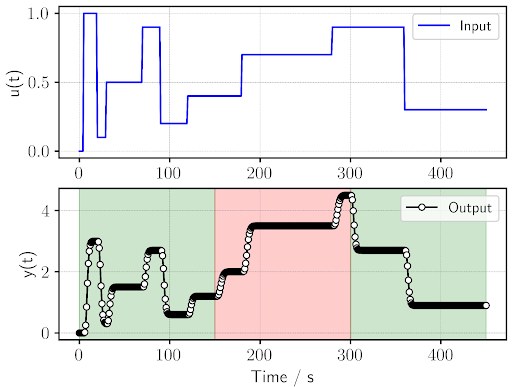
The following images show the plots of our input and output signals, where we can notice the time period of faulty operation at 150 - 300s in red and the stages of normal operation in green:
- Next the user decides on the appropriate system identification model, its parameters, and the time window used to sample data for identification. In our example, we are using an AutoRegressive with eXogenous inputs (ARX) model with 2 and 3 coefficients for its numerator and denominators, respectively. As for the time window, we define a window length of 80 s, which means that at every second of operation, we are processing a subset of 80 data points. The following code block, after defining the model parameters, loops over each second of the operation. On each loop, we retrieve the rolling window to be identified (defined as
data_subset) from the input-output signals defined earlier (defined asdata) and identify the system using Sippy’s built-in functionsystem_identification. Following system identification, we simply create the transfer function of our identified system,g_sample_subset, with the function tf from thecontrol.matlabpackage (defined ascnt), and use it to simulate the identified response,Y_ident_subset, for the entire time-span of operation by using thecntfunctionlsim.
window_length = 80
arx_numerator_order = 2
arx_denominator_order = 2

# For window length number of samples the coefficients will not be calculated
numerators = window_length * [
  arx_numerator_order * [0.0]]
denominators = window_length * [
   (arx_denominator_order + 1) * [0.0]]

Y_ident_timei = []

for i in range(0, ns - window_length):
  data_subset = data.iloc[0 + i : window_length + i, :]
  # SVD is failing if u is same value in the window and y changes
  # Putting in small noise to overcome it
  if (data_subset["u"] == data_subset["u"].iloc[0]).all():
       print("log: fixing same u values")
       # Add uniform random noise within +-1% amplitude of the base value
       base_val = data_subset["u"].iloc[0]
       data_subset["u"] = np.random.uniform(
           0.99 * base_val, 1.01 * base_val, data_subset.shape[0]
       )

  try:
      Id_ARX = sippy.system_identification(
          data_subset.y.to_numpy(),
          data_subset.u.to_numpy(),
          "ARX",
          centering="MeanVal",
          ARX_orders=[
              arx_numerator_order,
              arx_denominator_order,
              0,
          ],
      )
      g_sample_subset = cnt.tf(Id_ARX.NUMERATOR, Id_ARX.DENOMINATOR, sampling_time)
      # Append coefficients to list for plotting
      numerators.append(Id_ARX.NUMERATOR[0][0])  # Only for 1,1,0 ARX model
      denominators.append(Id_ARX.DENOMINATOR[0][0])
      # Log the parameters of the first window
      if i == 0:
          base_numerator = Id_ARX.NUMERATOR[0][0]
          base_denominator = Id_ARX.DENOMINATOR[0][0]
      # simulate with whole dataset
      Y_ident_subset, Time_subset, Xsim_subset = cnt.lsim(
          g_sample_subset, data.u.to_numpy(), data.time.to_numpy()
      )
      print(i)
      Y_ident_timei.append(Y_ident_subset)
  except:
      print(f"Failed on iteration {i}")
      numerators.append(None)
      denominators.append(None)

Y_ident_timei = np.transpose(np.asarray(Y_ident_timei))
num_df = pd.DataFrame(numerators)
den_df = pd.DataFrame(denominators)

# Plot customisation parameters
plt.rcParams['text.usetex'] = True

SMALL_SIZE = 8
MEDIUM_SIZE = 12
BIGGER_SIZE = 14
plt.rc('font', size=BIGGER_SIZE)          # controls default text sizes
plt.rc('axes', titlesize=BIGGER_SIZE)     # fontsize of the axes title
plt.rc('axes', labelsize=BIGGER_SIZE)    # fontsize of the x and y labels
plt.rc('xtick', labelsize=BIGGER_SIZE)    # fontsize of the tick labels
plt.rc('ytick', labelsize=BIGGER_SIZE)    # fontsize of the tick labels
plt.rc('legend', fontsize=MEDIUM_SIZE)    # legend fontsize
plt.rc('figure', titlesize=BIGGER_SIZE)  # fontsize of the figure title

# Plotting input and output variables as a function of time, highlighting normal and faulty operation
plt.figure()
ax1 = plt.subplot(2, 1, 1)
plt.setp(ax1.spines.values(), linewidth=1.3)
ax1.tick_params(width=1.3)
plt.grid(color = 'gray', linestyle = '--', linewidth = 0.25)
plt.plot(t, u, color = 'blue', label="Input")
plt.legend(["Input"], loc="best")
plt.ylabel("u(t)")

ax2 = plt.subplot(2, 1, 2)
plt.setp(ax2.spines.values(), linewidth=1.3)
ax2.tick_params(width=1.3)
plt.grid(color = 'gray', linestyle = '--', linewidth = 0.25)
plt.plot(t, yp_composite, color = 'black', marker = 'o', ms = 5, mec = 'k', mfc = 'white', label="Output")
plt.ylabel("y(t)")
plt.legend(loc="best")
plt.xlabel("Time / s")
ax2.axvspan(
   0,
   t_changepoint_low,
   alpha=0.2,
   color="green"
)
ax2.axvspan(
   t_changepoint_low,
   t_changepoint_high,
   alpha=0.2,
   color="red"
)
ax2.axvspan(
   t_changepoint_high,
   450,
   alpha=0.2,
   color="green"
)
plt.show()

# Plotting identified system at different rolling windows
plt.figure(2)
ax1 = plt.subplot(211)
plt.setp(ax1.spines.values(), linewidth=1.3)
ax1.tick_params(width=1.3)
plt.grid(color = 'gray', linestyle = '--', linewidth = 0.25)
plt.plot(data.time.to_numpy(), data.y.to_numpy(), color = 'black', marker = 'o', ms = 4, mec = 'k', mfc = 'white', label="Real y")

n = 8
colors = plt.cm.cool(np.linspace(0,1,n))

n2= 8
colors2 = plt.cm.jet(np.linspace(0,1,n2))

plt.plot(Time_subset, Y_ident_timei[:,1], color = colors[1],label=f"ID at 1s")
plt.plot(Time_subset, Y_ident_timei[:,130], color = colors[3],label=f"ID at 130s")
plt.plot(Time_subset, Y_ident_timei[:,350], color = colors[7],label=f"ID at 350s")
plt.ylabel("y(t)")
plt.ylim(-0.5, 8)
plt.legend(fontsize=9)
ax1.axvspan(
   t_changepoint_low,
   t_changepoint_high,
   alpha=0.2,
   color="red"
)

ax2 = plt.subplot(212)
plt.setp(ax2.spines.values(), linewidth=1.3)
ax2.tick_params(width=1.3)
plt.grid(color = 'gray', linestyle = '--', linewidth = 0.25)
plt.plot(((den_df.iloc[:,0] - base_denominator[0]) / base_denominator[0]) * 100, color = colors[1], linestyle = '-')
plt.plot(((den_df.iloc[:,1] - base_denominator[1]) / base_denominator[1]) * 100, color = colors[3], linestyle = '-')
plt.plot(((den_df.iloc[:,2] - base_denominator[2]) / base_denominator[2]) * 100, color = colors[7], linestyle = '-')
plt.ylim(-150,150)
plt.xlabel("Time / s")
plt.ylabel("Change in coeffs / \%")
plt.legend(["Den1","Den2","Den3"], loc="upper left",fontsize=9)
ax2.axvspan(
   t_changepoint_low,
   t_changepoint_high,
   alpha=0.2,
   color="red"
)

plt.show()
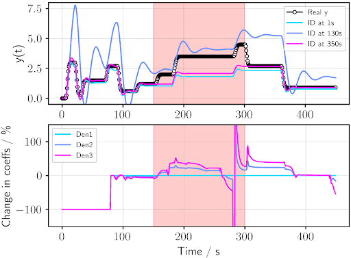
- The final step is to analyse the identified systems and evaluate how our asset is operating. The first plot of the following figure depicts the identified outputs at three interesting points in time. Taking a look at our identified signals at 1 and 350s, we can see very clearly that these are able to faithfully capture our real output from 0 to ~150s and from ~300 and onwards but appear to fail outside these time periods. This, together with the marked deterioration in our identification at all times at the 130-second point (which takes data before and after the fault at 150s), is an indication that something changed in the system at 150s and reverted back to its initial state at 300s. To confirm this, we plot the temporal evolution of the percentage change in the denominator coefficients of identification from those at t = 0s and notice how the time evolution of the second and third coefficients of the identified ARX model appear to exhibit a deviation from 0% at around 150s and a subsequent subsiding after 380s (once the rolling window of 80s does not contain any more of the data from the anomalous region of 150-300s).
Interestingly, the plot at the bottom exhibits noticeable spikes in the percentage change of the 2nd and 3rd denominator coefficients at ~280s, likely caused by the ARX model failing to converge. This is an indication that our SystID process requires more robust models or better parameter specification to avoid convergence issues that might lead to false failure flags. Considering the complexity of real-life operations, the choice of modelling strategies for SystID and anomaly detection becomes non-trivial, and perhaps as complex as the system itself. This is where an objective assessment of the available models and input parameter’s suitability to our specific use case comes into play—a task some might consider an art.
This small example of off-line SystID and fault detection allows us to see how we can easily adapt and expand these lines of code to reach the domains of more complex online and recursive problems. For instance, acquiring data of a collection of physical assets in real-time, streaming these data points into a platform that combines SystID, data-powered and physics-driven modelling, and identifying failures in their performance in a continuous manner. Such a task requires a combination of sensor technology to collect data from the physical assets and a sophisticated real-time connectivity framework. Through the Quaisr platform, scientists and engineers can easily create, lay-out, organise, interconnect, and consolidate different operation blocks—each with a particular task—to create a customised ensemble of coupled operations working towards specific goals.
Quaisr lets you reliably add complexity over time
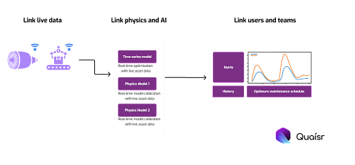
Quaisr links physics and AI
Connectivity can be taken further with Quaisr. Physics-based simulations have always played a pivotal role in decision making processes. Now engineers and scientists can supercharge simulations by linking them to live data and AI algorithms using the Quaisr platform.
Success relies on effective dialogue between two different teams, however a lack of standardisation and connectivity means that each team runs its own isolated process. Quaisr unlocks better maintenance decision-making pipelines linking simulation development with SystID practices. Quaisr helps users to iteratively increase the level of realism in a given model.
Simulation outputs are a key input for SystID blocks by enhancing pure data-driven time series with physics-informed models, providing a good trade-off between efficiency and accuracy. For instance, SystID algorithms working with turbulent boundary layer sensing data from a wind turbine airfoil could be informed via reduced order physics-encoding high-fidelity models to better identify and describe the pressure and shear-stress fluctuations accumulating at different sections of the airfoil. This information can be crucial later for adequate boundary layer separation control. Simultaneously, the SystID module would be receiving real-time input data and carrying out efficient optimisation calculations. Quaisr streaming capability means that users can always act in real time. Connectivity not only goes forward but can also close the loop to return new information, which can be used to re-adjust the simulations to better describe the physical asset based on real-time data acquisition. It may seem like years of development work is required to have such an interconnected system, but all of this can be achieved today using the Quaisr platform.
Quaisr links experts and non-experts
Quaisr provides a huge advantage to workflow connectivity, enabling users to promptly and smoothly couple different frameworks (e.g. data streaming, machine-learning and physics-based simulation/physics-encoding models) through the same drag-and-drop environment, augmenting overall process robustness and centralising your workflow development in a single platform. This methodology grants a high degree of accessibility to all aspects of the workflow, making them readily available for technical and non-technical users, empowering teams throughout your organisation by boosting their digital capabilities. Quaisr accompanies you and your organisation along your digitalisation journey.
Quaisr lets you collaborate and keep accountability
A key aspect when considering the added layers of complexity to a given workflow is traceability and version control. How to keep track of modifications in simulations, data-driven algorithms and data-acquisition protocols, all at the same time? Luckily, Quaisr integrates the necessary elements within its framework to guarantee governance and accountability. This puts an end to the frequent ‘Silo Mentality’. With Quaisr teams are connected and able to follow the workflow’s ongoing state and all previous iterations performed by other teams, completely cutting off the need to manually keep reports on past decisions and thus steadily reducing backlog issues. Version control and history are a key part of the Quaisr platform. Knowledge can be shared across all relevant areas of your organisation, providing an understanding of the current state of the process and preventing redundant or misaligned work which hinders the organisation’s agility and adaptability when it comes to decision making.
Key takeaways
- Quaisr links real-time data with modelling techniques to accelerate development of preventative maintenance workflows.
- Quaisr links physics- and ML-based models to increase the reliability of preventative maintenance frameworks.
- Quaisr keeps track of development efforts by building audit trails.