An engineer's guide to Active Learning: Training predictive models efficiently

Overview

Until recently, Active learning (AL) was one of those terms we'd heard multiple times from our data scientist colleagues and friends but struggled to relate to any of our day-to-day operations as engineers. This blog post sheds light on how active learning can transcend its reputation as a tool exclusive to the realm of cutting-edge data analysis and can become an essential asset in every engineer's toolkit. It also discusses how Quaisr can give you an easy but strong starting point to incorporate AL in your experiments and simulations, wherever your machine learning (ML) and coding knowledge is at the moment.

At the end of this blog, you will better understand:

• The general definition of active learning in machine learning
• The most common methods and strategies
• Its usefulness for us engineers, showcased through an engineering case study
• How Quaisr can help connect engineering expertise to active learning frameworks

Active Learning in Machine Learning – A General Definition

In its most general form, active learning is a collection of machine learning techniques and methods that revolve around strategic and interactive data selection for model training. In a nutshell, AL seeks to select only the best pieces of information to teach our models efficiently instead of just throwing a massive (and perhaps most importantly, very expensive) data set at the model and hoping for good performance.

The central idea behind AL is the recognition that not all data points in our sampling space hold equal importance. Therefore, our algorithms should possess the capability to strategically identify these 'high-value' points for labelling, aiming to improve the model's performance. This core concept, which can be summarised as 'not all data points are created equal,' proves especially valuable in a world where the process of data labelling can be incredibly costly and time-consuming, as you can see in this article. By carefully choosing which data to label, AL can optimise the learning process, reduce labelling expenses, expedite model convergence, and improve generalisation.

AL is actively used across a wide variety of interesting and exciting fields. Let's quickly explore some:

• Medical Diagnostics: AL is playing a pivotal role in advancing medical imaging techniques, including PET and CT scans, MRIs, and X-rays. AL algorithms are instrumental in identifying the most complex and uncertain cases. This targeted approach enhances the accuracy of diagnostic models, resulting in expedited and more reliable disease detection.

• Email Spam Filtering: Email spam filtering, particularly in large organisations, demands extensive, fully labelled datasets for effective classification and identification of suspicious emails. AL is useful in helping the models adapt to ever-changing spam patterns. Instead of relying solely on predefined rules, spam filters select uncertain or suspicious emails for human review, which helps refine filtering algorithms and reduce false positives.

• Document classification in legal procedures: Legal procedures, especially high-profile criminal trials, often unleash torrents of data in the form of evidence. AL steps in as a crucial ally for attorneys and legal professionals tasked with managing this staggering volume of information. By strategically reducing the number of documents requiring manual human review, AL streamlines legal processes and helps ensure the efficient administration of justice.

How does AL work?

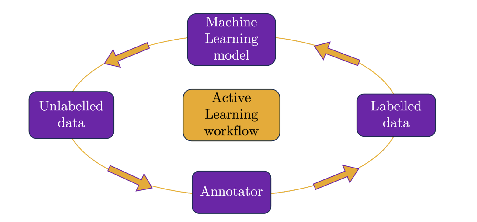
A general active learning (AL) workflow comprises four essential components in continuous interaction with each other: (i) The unlabelled dataset, (ii) The annotator (or 'oracle' in AL jargon), (iii) The labelled dataset, and (iv) The ML model.

The typical AL loop, as illustrated in the image below, starts with a small subset of labelled data, serving as the foundation to train an initial ML model to perform classification or regression tasks. Following this, the querying approach selected (more on this in just a moment) determines the specific data points requiring annotation, often involving a human annotator ('human-in-the-loop') to provide ground truth labels. As we will see next, in typical engineering applications the human annotator is replaced by different algorithms and simulations. From there, the ML model is updated, and its performance is evaluated. This iterative process is repeated until the loop's stopping criteria are met, which may include reaching a desired level of performance, a maximum number of labelling iterations, or a budget constraint for manual labelling. Finally, the updated model is tested with a new unlabelled dataset.

A quick note on notation: Throughout this blog post, we will use specific symbols to represent key elements. An individual data point will be denoted as $x^{(i)}$, its corresponding ground-truth label as $y^{(i)}$, and the label predicted by the ML model as $y^{*(i)}$. In classification tasks, $y^{*(i)}$ is the class or group to which $x^{(i)}$ belongs, while in regression tasks, $y^{*(i)}$ is typically the value of the function the ML is learning. Our unlabelled dataset is represented as $U=\{x^{(i)}, ?\}$ and our labelled dataset as $L=\{x^{(i)},y^{(i)}\}$.

The querying strategies used in AL can generally be embedded in three main scenarios, which can all be found in engineering problems. Let’s briefly explain each one:

• Pool-based sampling: These strategies are based on the existence of a large 'pool' of unlabelled data from which the sampling model selects a batch of $N$ informative points to be manually labelled. As we will see in the following sections, you can think of your large space of possible operating conditions of your system as a pool of unlabelled data.
• Stream-based selective sampling: This approach is specifically tailored for scenarios where unlabelled data arrive in a continuous stream. In this type of sampling, the AL system decides whether or not to ask for a label for each data point as it arrives in the stream.
• Query synthesis methods: Within this group of methods, the active learning system takes the initiative to synthetically generate unlabelled instances that it deems highly informative for subsequent labelling.

Common AL sampling methods

Now that we've laid the groundwork, you might be curious about how active learning systems go about selecting the most informative points for labelling. As is often the case in the world of data science, there's no shortage of methods and approaches, each with varying degrees of complexity, that have emerged over the years. In this blog post, we'll focus on the most relevant ones for common engineering problems.

Sampling strategies in active learning can be broadly categorised into three main classes based on the underlying 'philosophy' guiding their selection of the most 'worthy' points for labelling in both regression and classification tasks. These strategies differ in how they balance diversifying the response space versus reducing overall data uncertainty, essentially navigating the delicate trade-off between exploration and exploitation. These three main classes are

• Diversity-based sampling.
• Uncertainty-based sampling.
• Query–by-committee sampling.

Diversity-based sampling methods

As their name suggests, diversity-based methods seek to label those data points which maximise the diversity of the labelled or unlabelled spaces instead of concentrating on a small region of uncertainty. These methods are especially important when dealing with highly imbalanced datasets or when the initially labelled dataset is skewed toward a particular subset of the data.

Greedy sampling

Greedy sampling (GS) is a category of active learning methods primarily designed for pool-based regression problems, which, as we will see in the following section, are particularly relevant for us engineers. These methods aim to enhance regression models by diversifying either the sampled data points themselves (referred to as Greedy Sampling on Inputs, or GSx), the regression outputs they produce (Greedy Sampling on Outputs, or GSy), or a combination of both (Greedy Sampling on Inputs and Outputs, or iGS).

Problem statement for GS algorithms: Given a pool of $N$ unlabelled input data points, denoted as $\{x^{(i)}\}_{i=1}^N$, the goal is to select $K$ points for labelling. As mentioned in our note about notation, we use $y^{(i)}$ to refer to the ground-truth label for $x^{(i)}$ and $y^{*(i)}$ to its model estimation. The regressor is then tasked with building a model based on these $K$ labels to predict the output for the remaining $N-K$ data points.

• GSx: This algorithm seeks to maximise the distance between labelled and unlabelled points within the input space. Given its detachment from the regression outputs, this algorithm is easy to implement and has a low computational cost. The GSx algorithm begins by selecting the first point for labelling, strategically placed at the centroid of all $N$ data points in the input space. The remaining $K-1$ data points are chosen based on their distances in the input space from the already labelled points, represented here as $x^{(j)}$. The next point to label, represented by $x^{(n)}$, is then selected as the one with the largest minimum distance to the labelled points. This ensures that each newly labelled point contributes maximally to the overall diversity of the dataset.

  $d_x (x^{(i)}) = \min_j | x^{(i)}-x^{(j)} |$

  $x^{(n)} = \argmax_{x^{(i)}} d_x (x^{(i)})$

• GSy: In contrast to GSx, this approach focuses on diversifying the output space. The algorithm starts with a small number of already labelled instances ($K_0$), whose entries in the input space can be found using GSx. $K_0$ must be large enough to produce a reasonable starting-point regression model, typically recommended to be at least equal to the number of features in the input space. The next point to label is found similarly to GSx, but the distance function is computed between the predicted value for each unlabelled data point ($y^*(i)$) and the ground-truth label of the already-labelled points ($y^(j)$), as shown in the equation below:

  $d_y (x^{(i)}) = \min_j | y^{*(i)}-y^{(j)} |$

  $x^{(n)} = \argmax_{x^{(i)}} d_y (x^{(i)})$

• iGS: This algorithm aims to strike a balance between diversification in the input and output spaces. The selected point for labelling combines information from both distance functions, as shown in the following equation:

  $x^{(n)} = \argmax_{x^{(i)}} d_x (x^{(i)}) d_y (x^{(i)})$

Uncertainty-based sampling methods:

These methods are some of the most widely used across the AL spectrum. They prioritise data for labelling based on the points that are expected to reduce the model's uncertainty the most. In classification tasks, these data points will typically be those that lie close to the boundary of their specific group (also called classification hyperplane). Simply put, uncertainty-based sampling methods are effective when the goal is to improve the model's confidence and overall accuracy by focusing on the most challenging or ambiguous data points. A few common measures of uncertainty, $H$, in classification are the following:

• Least confidence: Using this measure of uncertainty, shown in the equation below, the sampler will select the instance $x^{(i)}$ that has the lowest probability of belonging to a class $y^{*(i)}$, $P(y^{*(i)} | x^{(i)})$:

  $H = \argmax_{x^{(i)} \in U} [ 1 - P(y^{*(i)}|x^{(i)})]$

• Margin sampling: Margin Sampling identifies the most uncertain point by comparing the probabilities of the top two predicted classes. The point with the smallest difference in probabilities is considered the most uncertain and challenging to classify:

  $H = \argmin_{x^{(i)} \in U} [ P(y^{*(i)}_{\{\text{best}\}}|x^{(i)}) - P(y^{*(i)}_{\{\text{second best}\}}|x^{(i)})]$

• Maximise entropy: Entropy is a popular uncertainty measure in ML. It essentially measures the level of disorder in the probabilities of the predicted classes. High entropy indicates that the probability distribution of a given data point over all possible classes is close to being uniform (i.e., it is highly uncertain to which class the point belongs to). These instances are chosen as they are expected to provide the most information for model improvement.

  $H = E_{x^{(i)}} = \argmin_{x^{(i)} \in U} \{ \sum_{y^{(i)} \in L} P (y^{*(i)}|x^{(i)}) \log P (y^{*(i)}|x^{(i)}) \}$

We should mention that these uncertainty-based methods for classification can also be adapted to regression tasks by adjusting the measures of uncertainty.

Query-by-committee sampling methods:

The last class of sampling methods we'll mention in this blog is Query-by-committee (QBC). Its core process is to create an ensemble of different classification models so that the uncertainty of a given point in the input space can be assessed individually by each member of this 'committee' of models. The selected point for labelling will typically be the one that produces the most disagreement between models as this is considered the most informative point for improving predictions. QBC tends to attenuate some of the problems exhibited by uncertainty-based methods given that the results are not biassed toward a specific model. Various criteria are used to measure the disagreement between committee members, including entropy-based measures, KL divergence, margin-based measures, and variability-based measures.

Why and how AL is relevant for engineers?

Now that we have a grasp of the general AL workflow and the most common sampling methods, it's time to address the question that might be on your mind: "How does active learning actually connect with my day-to-day work as an engineer? How can it enhance my simulations and experiments?" Let's bridge the gap and see how AL aligns with our engineering workflows, whether they involve optimising the performance of a chemical plant, accelerating product development, efficiently performing preventative maintenance, or simply getting more out of your simulations.

Envision the pool of unlabelled data we've been discussing in this blog as a specific collection of operating conditions that we urgently need to explore within our system of interest. Similarly, consider the process of data labelling as akin to conducting expensive experiments or simulations to obtain the system's response for every single instance within our pool of conditions and hopefully build a useful model of our system. By framing the general problem statement of AL in this context, we can readily understand its direct relevance to engineers.

Strategically selecting only the most informative operating condition values for conducting experiments and simulations, rather than attempting to cover the entire spectrum, not only translates into substantial resource savings but also holds the promise of achieving better model performance. This streamlined approach not only sharpens our decision-making but also proves invaluable when contending with those lengthy, time-consuming experiments and simulations that are all too familiar to us engineers.

As engineers who have dealt with high-fidelity Direct Numerical Simulations (DNS) for multiphase flows in the past, we've personally experienced the frustration of waiting for months to obtain results from a single simulation, only to discover that they bear little deviation from the outcomes of previous simulations. This is a scenario engineers often encounter, and it's precisely where an effective AL framework comes to the rescue, significantly reducing the likelihood of such disappointments and wasted resources.

Where does Quaisr come into play?

The answer is quite straightforward: enabling engineers and researchers to connect and integrate AL methods into their workflows. Let us speak from our own experience.

We are currently final year engineering PhD students at Imperial College London. Our day consists pretty much exclusively of running high-fidelity, physics-encoding CFD simulations and connecting their outputs to ML and deep learning models to develop cheaper data-driven surrogate predictors that can speed up decision-making pipelines in industrial and commercial scenarios. Given the nature of our in-house CFD code, each run is extremely time-intensive and computationally demanding, even with access to Imperial College's High Performance Computing (HPC) resources. As a result, generating sufficient high-quality data for training neural networks and other ML algorithms poses a significant challenge for us.

In our computational lab, we are surrounded by other brilliant PhDs who face a similar problem to us. To ease our burden, we developed from the ground up an automated system that allows us to generate, orchestrate, and post-process physics-based simulations at Imperial College's HPC. It took us more than a month of software development to get a stable framework that successfully submits and processes simulation runs automatically (admittedly, we are engineers, not software developers). However, this only solves half of our issues, as our code currently operates with a space-filling LHS model to generate our simulation's sample space, and the CFD results extracted from each run have to be manually transferred into our ML workflow.

Our next challenge would be to replace the static LHS sampling method with an AL technique, and directly plug our simulations’ output into our ML workflow, which will take us who knows how long to code!

These challenges could be easily fixed through a Quaisr platform deployment. Deploying, connecting and orchestrating a large number of simulation and ML runs would take less than a day, and could be easily tailored to any type of CFD software, whether it is our in-house code, or something more widely used like OpenFOAM.

What is more interesting is that Quaisr could allow us to build applications for our supervisor to access and see analysis outcomes as soon as they become available. Weekly meetings could be superseded by real-time updates through the Quaisr app, easily saving us at least 5 hours a week for preparing and attending meetings.

What's more, the Quaisr platform would grant easy and transparent collaboration with our other PhD colleagues. No need to have extra impromptu meetings to make sure the right Git commit and branch merge goes through or that a crucial addition to the code is not lost! Experimentation becomes easy with Quaisr, with a log of past outcomes being saved and readily available to all users, facilitating decisions as to what works and what doesn't.

With Quaisr, we will not need an extra month or two of arduous coding and software development to get our CFD framework up and running with AL methodologies, or to get direct feedback from our surrogate model’s performance based on the CFD simulations that are being processed. All of this can be done on the spot from the same environment.

But let's get back on topic: Active Learning and how it helps us train predictive models faster. Below is an example where we use a physics-based numerical solver and train a predictive model.

A case study of an engineering problem

Let's consider a simple scenario in structural engineering: stress analysis. Our objective is to assess a beam's maximum deformation before failure based on two crucial factors: its length, $L$, and a measure of the material's elasticity, . This entails solving the following PDE which governs small linear elastic deformations of a body:

$\mathbf{\sigma} = \lambda (\nabla\cdot \mathbf{u}) \mathbf{I} + \mu [\nabla \mathbf{u} + (\nabla \mathbf{u})^\intercal]$

where $\mathbf{\sigma}$ is the stress tensor, $\lambda$ and $\mu$ are intrinsic elasticity parameters for each material, $\mathbf{I}$ is the identity tensor, and $\mathbf{u}$ is the displacement vector field. Even though it only takes us a single page of code to implement a Finite Element Method (FEM) discretisation strategy to solve this problem in an open-source platform like FEniCS (read more here), lets imagine FEM calculations are the equivalent of high-end, costly physics-encoding simulations. Traditional engineering practices would seek to implement a process as detailed below:

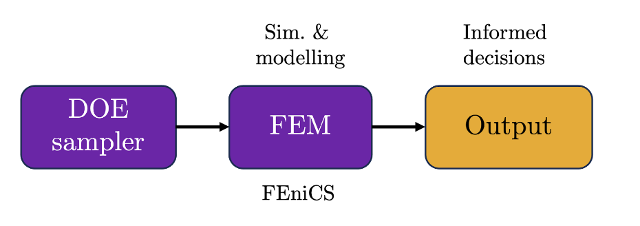
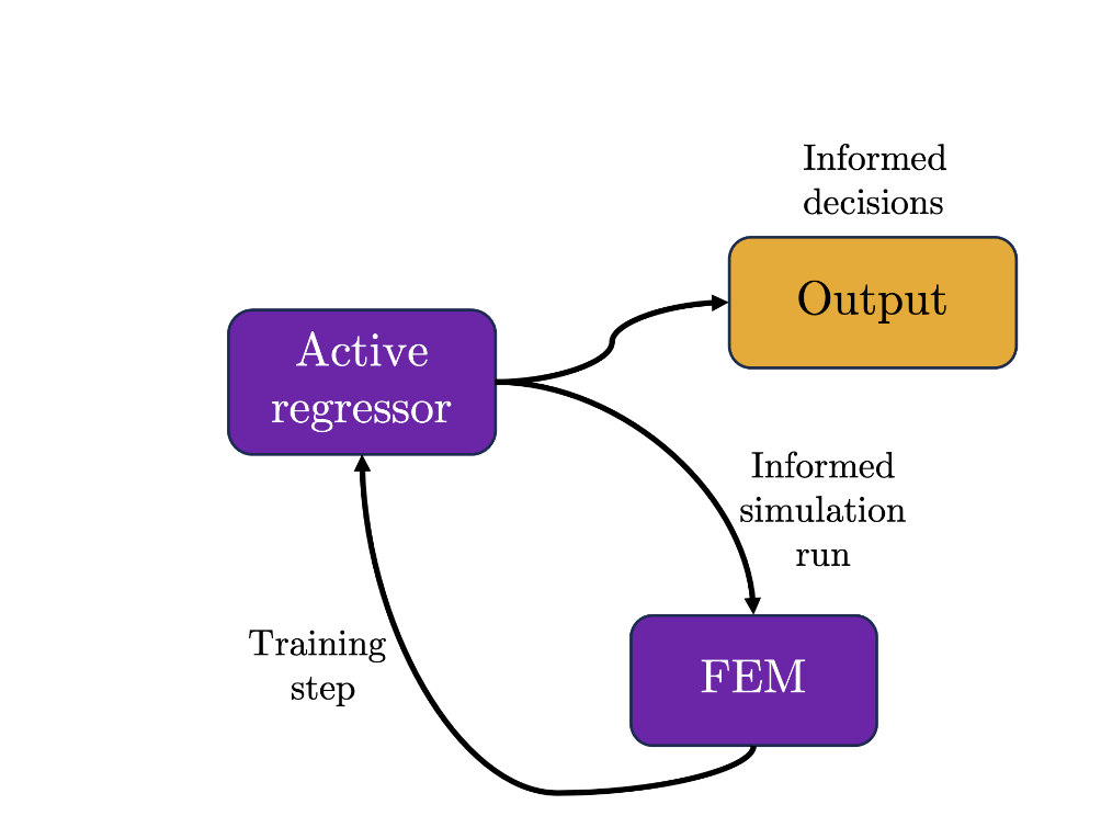
A design of experiments (DOE) method would be used to generate the initial set lengths $L$ and elasticities $\mu$ to run through the FEM simulator and after weeks or even months of run time and arduous post-processing, informed decisions would be possible. However, if our initial problem statement evolves or is altered in any way, we would need to drive back to step one and run the whole process again. Nowadays, these operations are slightly more sophisticated and leverage the power of data-driven algorithms to train cheaper surrogate models from high-fidelity simulation data, thus providing informed decisions significantly faster, and ultimately aiming to replace time-consuming and costly simulation workflows altogether. This new pipeline would be as follows:

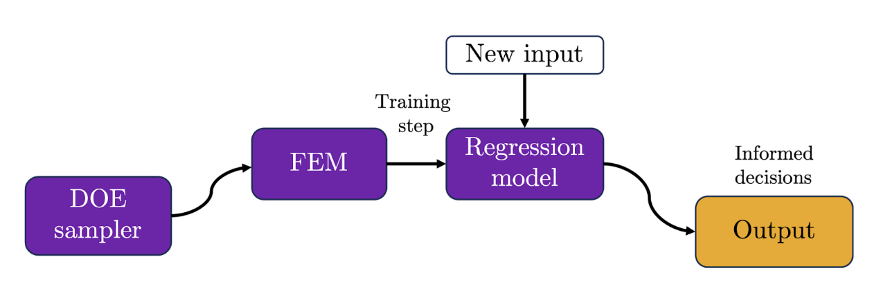
Despite being an improvement from the early trial and error approach, a new problem arises in the adequate training of such surrogate models. Once again, it seems we might need numerous high-fidelity simulations to attain a sufficiently accurate surrogate that can effectively replace modelling efforts, rendering an equally costly and time-consuming process. Besides, there is no guarantee that key physical mechanisms (e.g., linear dependency between stress $\mathbf{\sigma}$ and deformation gradients $\mathbf{u}$) will be appropriately captured by our surrogate model, casting doubt over its interpretation and prediction over unseen or critically different scenarios. So, what next?

Instead of simulating a random batch of DOE-generated cases, we can plug FEM simulations directly into an active regressor, which intelligently chooses the next set of $(L, \mu)$ values to simulate based on the current training state of the surrogate predictor. In this way, active regressors efficiently avoid flat or uninteresting regions in our sample $(L, \mu)$ space, thus reducing the number of simulations and training efforts required to attain a high level of accuracy. As we mentioned before, the active regressor acts as a labeller by selecting the next conditions to simulate from the pool of unlabelled cases. As we explored previously, depending on the sampling technique selected for the AL algorithm (e.g., greedy sampling on the input, etc), the active regressor quickly locates the region of interest within the sample space, and assesses the balance between exploiting a known region or exploring areas farther away within the sample space, based on its pre-defined objective function (i.e., exploitation vs. exploration).

Naturally, this approach provides a wide range of applicability due to its flexibility in accommodating target-oriented objective functions, essentially generating a sampling route tailored for any type of parameter space. In this way, uncertainty in the sample space is reduced and faster convergence toward the region of interest can be ensured, leading to a highly efficient training process that ultimately yields more robust surrogate models.

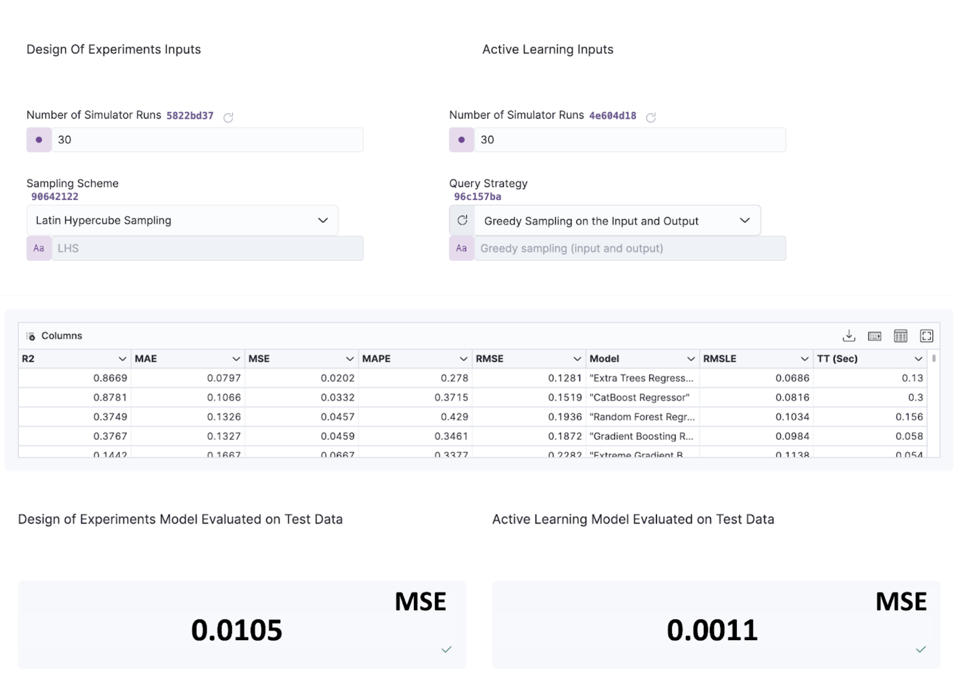
The Quaisr platform allows us to immediately compare both approaches (e.g., DOE vs. active sampling) and visualise the impact of the active regressor in the pipeline shown above. It is as simple as swapping our sampling block into the pipeline, whilst maintaining the same FEM simulation algorithm. Let's first consider an equal number of FEM runs to be used as training data for our surrogate, and compare the points probed by both the AL (using iGS) and DOE (using Latin Hypercube Sampling, refer to our previous blog) sampling algorithms in the $(L, \mu)$ space.

First, we compare the performance by comparing surrogate predictions from AL (using iGS) and DOE (using Latin Hypercube Sampling, refer to our previous blog) for an equal set of 30 $(L, \mu)$ pairs. The trained surrogate resulting from the AL-selected FEM simulations performs significantly better than its DoE counterpart despite using the same amount of training data, yielding a Mean-Squared Error nearly ten times smaller than that obtained for the DOE-trained model, as appreciated below:

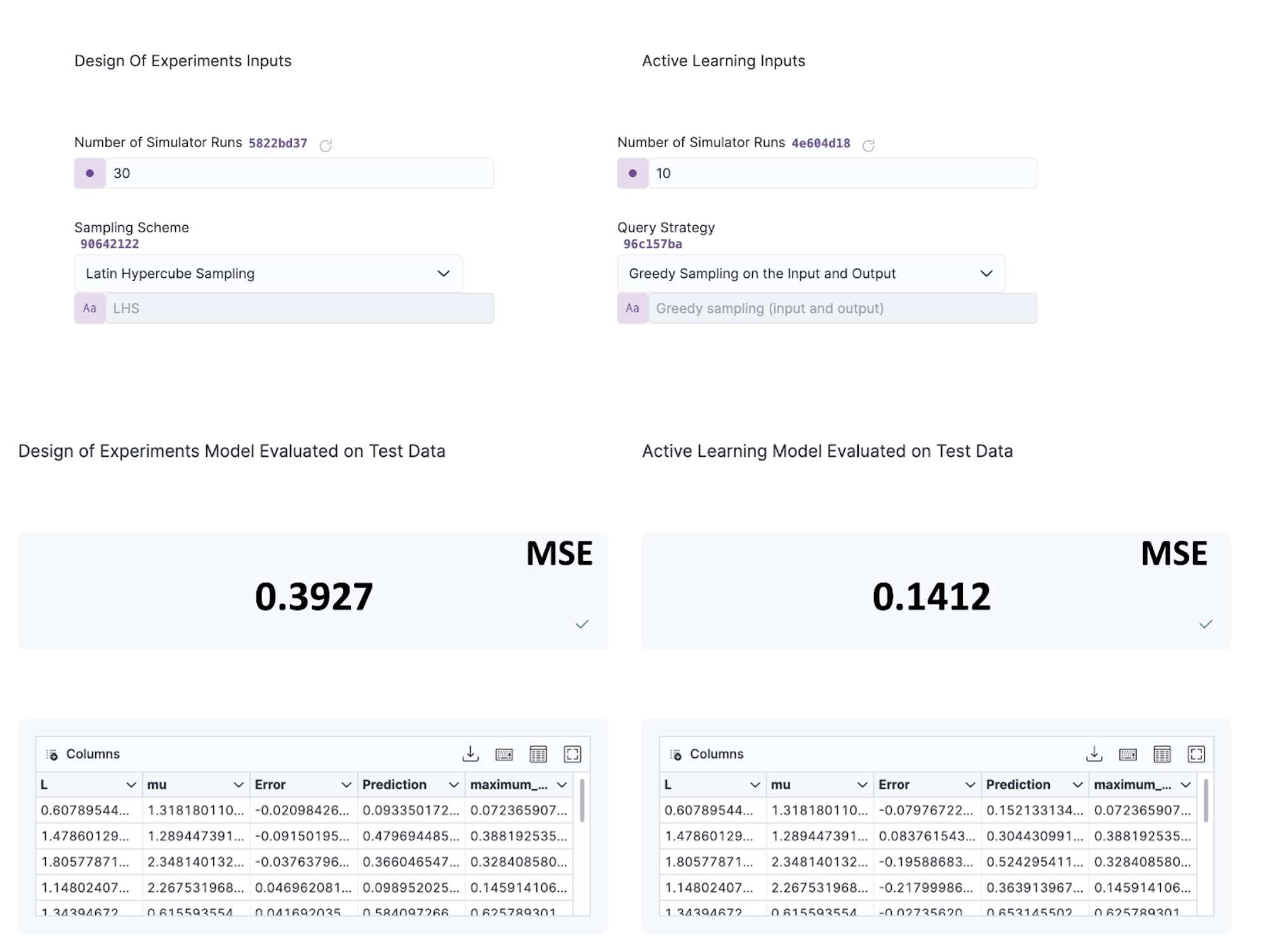
Even with 2/3 less data to train from, the active regressor yields a lower MSE than its DOE counterpart when subjected to the same 10 $(L, \mu)$ testing points, demonstrating the huge potential behind active regressors.

Tackling complex engineering scenarios

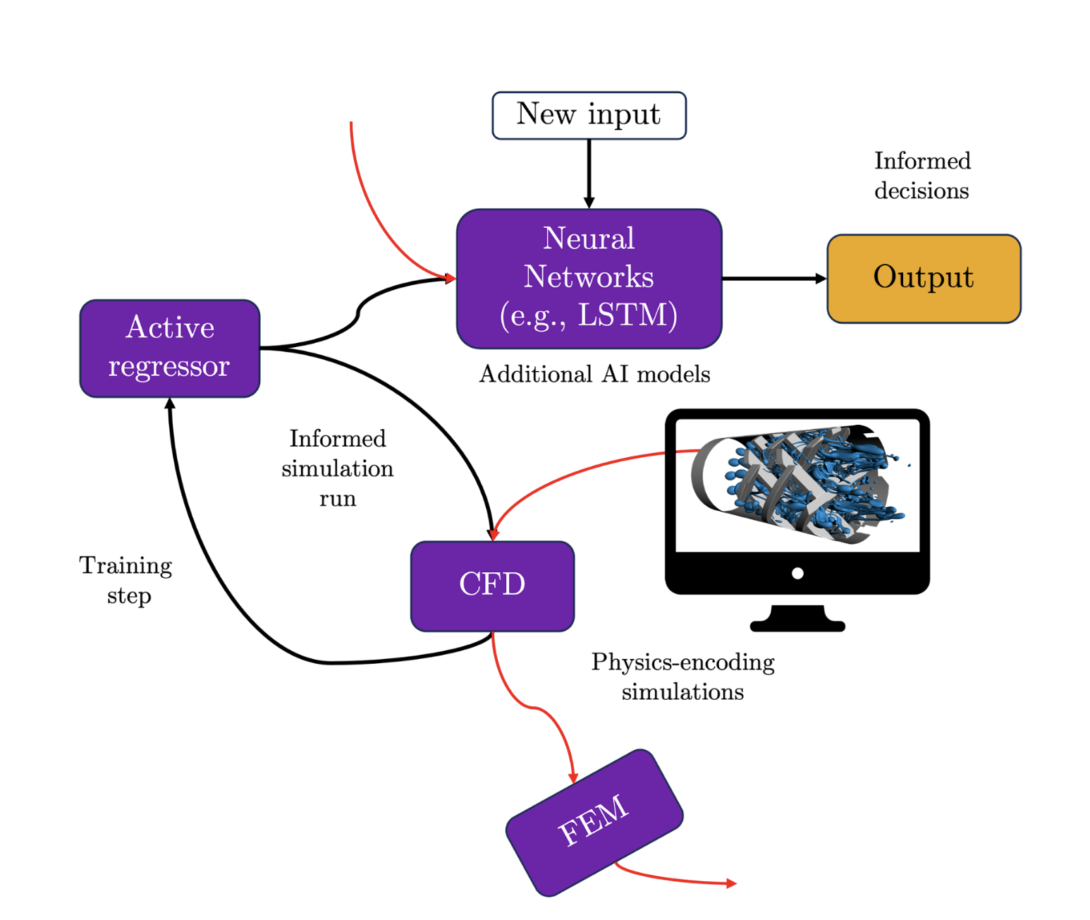
The Quaisr platform allows us to switch between different sampling techniques (whether it is traditional DOE or more sophisticated AL approaches), and fine-tune each method with as much detail as required (e.g., built-in, or user-defined DOE schemes and AL query strategies), rendering the ultimate tool, tailored on the fly for any scenario. Similarly, we can increase the complexity of our workflow by simply swapping our FEM block with any other Python library, software package or simulation model we might need, and still perform the same sample space exploration with no further coding or modifications required in our workflow. Let’s explore a hypothetical, more complex scenario in mixing systems for the FMCG and pharmaceutical industries to visualise just how easily Quaisr can adapt to new scenarios.

Imagine our objective is to find the best geometrical features and operational conditions for a given mixing process based on either experimental or simulation runs. Nowadays, experimental trial runs are costly and frequently conflict with environmental and sustainability goals, given the need to handle waste material after each run. Consequently, Computational Fluid Dynamics (CFD) simulations are the most logical, yet not necessarily the cheapest alternative, given the highly robust models needed to account for numerous intricacies that accompany industrial scale mixing systems (e.g., non-Newtonian rheology, turbulence, interfacial and multiphase modelling, and the list goes on and on). Once again, it seems we need to develop and fine-tune AI tools that can do the heavy lifting and minimise our dependence on computationally expensive simulations.

With Quaisr, there is no need to build a new workflow around our high-fidelity CFD model, we can simply adapt the initial pipeline tested above by swapping the FEM simulator block with our CFD code. The best part? This new block can be commercial, open-source or in-house CFD code, We can add further complexity as required to our pipeline, such as deep-learning models (e.g., Long-Short-Term Memory (LSTM) recurrent neural networks to deal with temporal problems) to complement or replace our simpler regression models. These more complex AI frameworks could immediately benefit from the advantages explored earlier with AL algorithms, undergoing an efficient and robust training process which minimises the need for CFD runs. In this way, we could carry out crucial predictions, such as temporal forecasting of mixing performance, without costly CFD runs, expediting the decision-making process. It seems like years of development and coding are required to achieve this, but a pipeline as shown below can be developed today with the Quaisr platform. And we can do it collaboratively!